Volumetric Analysis with UAS

Introduction

Conducting Volumetric Analysis with UAS imagery is a valuable and useful tool for many companies and operations. Ongoing or periodical analysis of stock piles of material will allow a business to work more efficiently and be more aware of their available material. We can conduct "cut" and "fill" operations for piles and for holes/ ditches to measure the volume of the mission area. It is very important when calculating volumetric data to have an accurate and consistent ground control points through the mission area. It is also important to have an accurate base elevation for the data, errors with the ground control points or the base elevation will result in processing errors or errors in the data that has been produced. UAS and aerial data is effective to use when creating volumetric calculations when done correctly, allowing the user to create accurate othomosiacs of the data and have a consistent geographic coordinate system throughout all of the data. Through this lab we were able to use Pix4D volumetric calculations as well as ArcMap calculations and were able to compare the two and see where the shortfalls were in each. 

Method

Wolfpaving Site

Pix4D

Volumetric calculations were initially done using Pix4D, Pix4D allows for quick an accurate volume calculations using the volumes tool located on the side tool bar. Upon completion of image processing and generation of the point cloud and orthomosiac we can calculate the volumes of the 3 designated stock piles pictured in Figure 1. 

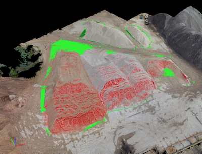Figure 1: Stock Piles

Using the Volumes tool we can trace around the desired stock pile and calculate the volume, it is important to have the correct base elevation to calculate volumetric data. The figures below show the designated stock piles and their corresponding volume calculations.

Figure 2: Stock Pile A

Figure 3: Stock Pile A Volume

Stock Pile A had a total volume of 469.47 cubic meters. 

Figure 4: Stock Pile B

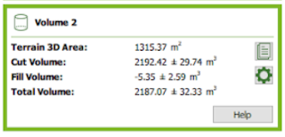Figure 5: Stock Pile B Volume

Stock Pile B had a volume of 2187.07 cubic meters. 

Figure 6: Stock Pile C

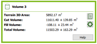Figure 7: Stock Pile C Volume

Stock Pile C had a volume of 11,503.29 cubic meters. 

ArcMap

Calculating volumes in ArcMap has 3 major steps; creating a feature class, extracting by mask and then calculating the volume. Once the UAS data for the Wolfpaving site has been added into ArcMap we can begin by creating a feature class for each of the stock piles. The created polygon features for stock piles A, B and C are pictured in Figure 8. 

Figure 8: Stock Pile Feature Class

Once the feature class has been created we are able to extract that areas specific data by a clipping mask which is the created polygon feature, Figure 9 shows the clipped Stock Pile A after performing an Extract by Mask. We will perform this step for each individual stock pile. 

Figure 9: Extract By Mass

After performing an extract by mass on each of the stock piles we can now calculate the surface volume for each of the stock piles. Here it is very important to input the correct base elevation when performing the calculations. Figures 10, 11 and 12 show the calculated volumes of stock piles A, B and C. 

Figure 10: Pile A Volume

Pile A had a calculated volume of 693.39 cubic meters. 

Figure 11: Pile B Volume

 Pile B had a volume of 2566.25 cubic meters. 

Figure 12: Pile C Volume

Pile C had a volume of 13,766.06 cubic meters. 

Figure 13: Wolfpaving Map 

Figure 13 pictures the 3 stock piles that were calculated at the Wolfpaving site.

Discussion 

By comparing the Pix4D and the ArcMap volumetric calculations we can see some significant differences in the calculated volumes. In Pix4D Pile A measured 469 cubic meters while ArcMap calculated it to be 693 cubic meters, a difference of around 200 cubic meters. Pile B was calculated to be 2187 cubic meters in Pix4D and 2566 cubic meters in ArcMap, a difference of around 400 cubic meters. Pile C was calculated to be 11,503 cubic meters with Pix4D and 13,766 cubic meters in ArcMap, a difference of around 2,000 cubic meters. As we went up in the overall pile volume we began to see a larger margin of error between Pix4D and ArcMap. There are many possible reasons for these errors including but not limited to; the base elevation, the drawn outline of the stock piles

and the ground control points. By running the volume calculation of Pile C in ArcMap with a 1 meter difference in base elevations I was able to see the difference in the calculations that only 1 meter would make, some were more significant than others totaling in around 1000 cubic meters. The ground control points as always can be inherently problematic if not used correctly in the data set.

Litchfield Site 

For the Litchfield dredging operation we performed the same steps in ArcMap that we did with the Wolfpaving site, but will resample the data to 10 cm before calculating the volume. Resampling the data will allow us to keep the data consisted over the 3 volumetric calculations we will take. The Litchfield calculations show the changes of the dredging stock pile over the span of three months, calculations were taken on July 22nd, August 27th and September 30th. Figure 14 and 15 below show the resampled clipped July 22nd extracted by mask feature of the dredge, along with the volume calculations. 

Figure 14: July 22nd Resampled Clip

Figure 15: July 22nd Volume

On July 22nd the dredge pile had a volume of 40,431.95 cubic meters.

Figure 16: August 27th Resampled Clip

Figure 17: August 27th Volume

On August 27th the dredge pile had a volume of 84,447.25 cubic meters,

Figure 18: September 30th Resampled Clip

Figure 19: September 30th Volume

On September 30th the dredge pile had a volume of 51,538.82 cubic meters. 

Discussion 

Figure 20: Litchfield Map

Figure 20 represents the three different dates that volume had been measured at the Litchfield dredging site. We are able to see the differences in the physical size and volumes of the three piles. We can compare these images with the data in Table 1 below. 

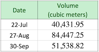Table 1: Litchfield Volumes

Through this data and the map we are able to compare and analyze the different volumes contained in this pile throughout the 3 months that it was observed, with July being the lowest volume and August being the highest. The data had been resampled to 10cm so all data is consistent throughout. The base elevation chosen for these calculations was 234 meters. I was able to run the volumetric of the three piles at different base elevations which resulted in numbers nearly 10,000 cubic meters different. The base elevation is a very important detail to make sure the data is consistent and accurate. It is important to ensure consistency throughout these calculations in order to have accurate data regarding the volume of the stock piles. Companies need to rely on this data in order to track their progress. We can visually see from Figure 20 where there are net gains and loses in the stock pile. Errors could have been encountered with the clip that was used for each pile, we can question if the clips covered enough area and captured all of the intended volume.

Conclusion

Volumetric data and analysis allows companies to consistently track and analyze their resources, materials and progress. Accurate volumetric data lets companies run more efficiently and consume their materials at a reasonable rate. It will also let them know if they are ahead or behind schedule on operations. UAS data is very useful when conducting volumetric calculations. Geo-referenced aerial data allows for accurate calculations and precise measurements.